Definitions and some radiation theory¶

In radiation physics there is unfortunately several slightly different ways of presenting the theory. For instance, there is no single custom on the mathematical symbolism, and various different non SI-units are used in different situations. Here we present just a few terms and definitions with relevance to PySpectral, and how to possible go from one common representation to another.

Symbols and definitions used in PySpectral¶

$\lambda$ Wavelength ( $\mu m$ )

$\nu = \frac{1}{\lambda}$ Wavenumber ( $cm^{-1}$ )

$\lambda_{c}$ Central wavelength for a given band/channel ( $\mu m$ )

$\nu_{c}$ Central wavelength for a given band/channel ( $cm^{-1}$ )

$\Phi_{i}(\lambda)$ Relative spectral response for band $i$ as a function of wavelength

$E_{\lambda}$ Spectral irradiance at wavelength $\lambda$ ( $W/m^2 \mu m^{-1}$ )

$E_{\nu}$ Spectral irradiance at wavenumber $\nu$ ( $W/m^2 (cm^{-1})^{-1}$ )

$B_{\lambda}$ Blackbody radiation at wavelength $\lambda$ ( $W/m^2 \mu m^{-1}$ )

$B_{\nu}$ Blackbody radiation at wavenumber $\nu$ ( $W/m^2 (cm^{-1})^{-1}$ )

$L_{\nu}$ Spectral radiance at wavenumber $\nu$ ( $W/m^2 sr^{-1} (cm^{-1})^{-1}$ )

$L_{\lambda}$ Spectral radiance at wavelength $\lambda$ ( $W/m^2 sr^{-1} \mu m^{-1}$ )

$L$ Radiance - (band) integrated spectral radiance ( $W/m^2 sr^{-1}$ )

Constants¶

$k_B$ Boltzmann constant ( $1.3806488 1e−23$ )

$h$ Planck constant ( $6.62606957 1e-34$ )

$c$ Speed of light in vacuum ( $2.99792458 1e8$ )

Central wavelength and central wavenumber¶

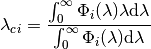
The central wavelength for a given spectral band ( $i$ ) of a satellite sensor is defined as:

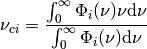
${\lambda_c}_i = \frac{\int_0^\infty \Phi_{i}(\lambda) \lambda \mathrm{d}\lambda} {\int_0^\infty \Phi_{i}(\lambda) \mathrm{d}\lambda}$

Likewise the central wavenumber is:

${\nu_c}_i = \frac{\int_0^\infty \Phi_{i}(\nu) \nu \mathrm{d}\nu} {\int_0^\infty \Phi_{i}(\nu) \mathrm{d}\nu}$

And since $\nu = 1/\lambda$ , we can express the central wavenumber using the spectral response function expressed in wavelength space, as:

${\nu_c}_i = \frac{\int_0^\infty \Phi_{i}(\lambda) \frac{1}{\lambda^{3}} \mathrm{d}\lambda} {\int_0^\infty \Phi_{i}(\lambda) \frac{1}{\lambda^{2}} \mathrm{d}\lambda}$

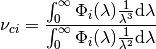
And from this we see that in general $\nu_c \neq 1/\lambda_c$ .

Taking SEVIRI as an example, and looking at the visible channel on Meteosat-8, we see that this is indeed true:

>>> from pyspectral.rsr_reader import RelativeSpectralResponse
>>> from pyspectral.utils import convert2wavenumber, get_central_wave
>>> seviri = RelativeSpectralResponse('Meteosat-8', 'seviri')
>>> cwl = get_central_wave(seviri.rsr['VIS0.6']['det-1']['wavelength'], seviri.rsr['VIS0.6']['det-1']['response'])
>>> print(round(cwl, 6))
0.640216
>>> rsr, info = convert2wavenumber(seviri.rsr)
>>> print("si_scale={scale}, unit={unit}".format(scale=info['si_scale'], unit=info['unit']))
si_scale=100.0, unit=cm-1
>>> wvc = get_central_wave(rsr['VIS0.6']['det-1']['wavenumber'], rsr['VIS0.6']['det-1']['response'])
>>> round(wvc, 3)
15682.622
>>> print(round(1./wvc*1e4, 6))
0.637648

In the PySpectral unified HDF5 formated spectral response data we also store the central wavelength, so you actually don’t have to calculate them yourself:

>>> from pyspectral.rsr_reader import RelativeSpectralResponse
>>> print("Central wavelength = {cwl}".format(cwl=round(seviri.rsr['VIS0.6']['det-1']['central_wavelength'], 6)))
Central wavelength = 0.640216

Spectral Irradiance¶

We denote the spectral irradiance $E$ which is a function of wavelength or wavenumber, depending on what representation is used. In PySpectral the aim is to support both representations. The units are of course dependent of which representation is used.

In wavelength space we write $E(\lambda)$ and it is given in units of $W/m^2 \mu m^{-1}$ .

In wavenumber space we write $E(\nu)$ and it is given in units of $W/m^2 (cm^{-1})^{-1}$ .

To convert a spectral irradiance $E_{\lambda_0}$ at wavelengh $\lambda_0$ to a spectral irradiance $E_{\nu_0}$ at wavenumber $\nu_0 = 1/\lambda_0$ the following relation applies:

$E_\nu = E_\lambda \lambda^2$

And if the units are not SI but rather given by the units shown above we have to account for a factor of 10 as:

$E_\nu = {E_\lambda \lambda^2 * 0.1}$

TOA Solar irridiance and solar constant¶

First, the TOA solar irradiance in wavelength space:

>>> from pyspectral.solar import (SolarIrradianceSpectrum, TOTAL_IRRADIANCE_SPECTRUM_2000ASTM)
>>> solar_irr = SolarIrradianceSpectrum(TOTAL_IRRADIANCE_SPECTRUM_2000ASTM, dlambda=0.0005)
>>> print("Solar irradiance = {}".format(round(solar_irr.solar_constant(), 3)))
Solar irradiance = 1366.091
>>> solar_irr.plot('/tmp/solar_irradiance.png')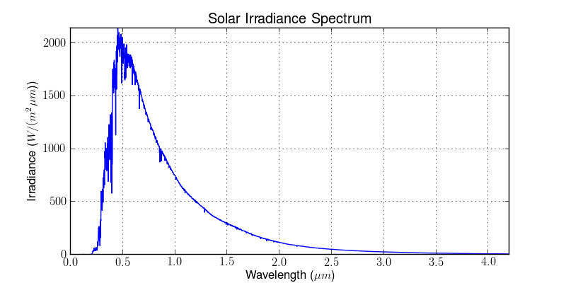

The solar constant is in units of $W/m^2$ . Instead when expressing the irradiance in wavenumber space using wavenumbers in units of $cm^{-1}$ the solar flux is in units of $mW/m^2$ :

>>> solar_irr = SolarIrradianceSpectrum(TOTAL_IRRADIANCE_SPECTRUM_2000ASTM, dlambda=0.0005, wavespace='wavenumber')
>>> print(round(solar_irr.solar_constant(), 5))
1366077.16482
>>> solar_irr.plot('/tmp/solar_irradiance_wnum.png')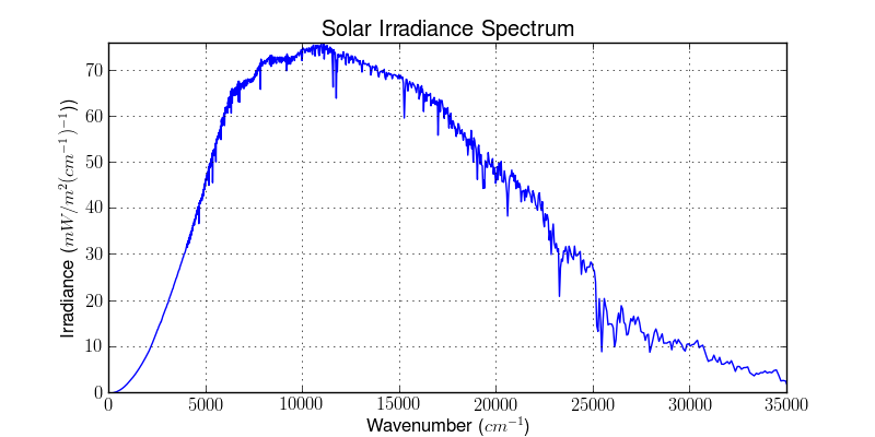

In-band solar flux¶

The solar flux (SI unit $\frac{W}{m^2}$ ) over a spectral sensor band can be derived by convolving the top of atmosphere solar spectral irradiance and the sensor relative spectral response. For band $i$ :

$F_i = \int_0^\infty \Phi_{i}(\lambda) E(\lambda) \mathrm{d}\lambda$

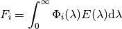
where $E(\lambda)$ is the TOA spectral solar irradiance at a sun-earth distance of one astronomical unit (AU).

In python code it may look like this:

>>> from pyspectral.rsr_reader import RelativeSpectralResponse
>>> from pyspectral.utils import convert2wavenumber, get_central_wave
>>> seviri = RelativeSpectralResponse('Meteosat-8', 'seviri')
>>> rsr, info = convert2wavenumber(seviri.rsr)
>>> from pyspectral.solar import (SolarIrradianceSpectrum, TOTAL_IRRADIANCE_SPECTRUM_2000ASTM)
>>> solar_irr = SolarIrradianceSpectrum(TOTAL_IRRADIANCE_SPECTRUM_2000ASTM, dlambda=0.0005, wavespace='wavenumber')
>>> print("Solar Irrdiance (SEVIRI band VIS008) = {sflux:12.6f}".format(sflux=solar_irr.inband_solarflux(rsr['VIS0.8'])))
Solar Irrdiance (SEVIRI band VIS008) = 63767.908405

Planck radiation¶

Planck’s law describes the electromagnetic radiation emitted by a black body in thermal equilibrium at a definite temperature.

Thus for wavelength $\lambda$ the Planck radiation or Blackbody radiation $B({\lambda})$ can be written as:

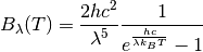
$B_{\lambda}(T) = \frac{2hc^{2}}{{\lambda}^{5}} \frac{1} {e^{\frac{hc}{\lambda k_B T}} - 1}$

and expressed as a function of wavenumber $\nu$ :

$B_{\nu}(T) = 2hc^2{\nu}^3 \frac{1}{e^{\frac{h c \nu}{k_B T}} - 1}$

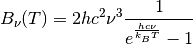
In python it may look like this:

>>> from pyspectral.blackbody import blackbody_wn
>>> wavenumber = 90909.1
>>> rad = blackbody_wn((wavenumber, ), [300., 301])
>>> print("{0:7.6f} {1:7.6f}".format(rad[0], rad[1]))
0.001158 0.001175

Which are the spectral radiances in SI units at wavenumber around $909 cm^{-1}$ at temperatures 300 and 301 Kelvin. In units of $mW/m^2 (cm^{-1})^{-1}\ sr^{-1}$ this becomes:

>>> print("{0:7.4f} {1:7.4f}".format((rad*1e+5)[0], (rad*1e+5)[1]))
115.8354 117.5477

And using wavelength representation:

>>> from pyspectral.blackbody import blackbody
>>> wvl = 1./wavenumber
>>> rad = blackbody(wvl, [300., 301])
>>> print("{0:10.3f} {1:10.3f}".format(rad[0], rad[1]))
9573178.886 9714689.259

Which are the spectral radiances in SI units around $11 \mu m$ at temperatures 300 and 301 Kelvin. In units of $mW/m^2\ m^{-1} sr^{-1}$ this becomes:

>>> print("{0:7.5f} {1:7.5f}".format((rad*1e-6)[0], (rad*1e-6)[1]))
9.57318 9.71469

The inverse Planck function¶

Inverting the Planck function allows to derive the brightness temperature given the spectral radiance. Expressed in wavenumber space this becomes:

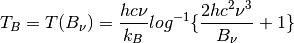
$T_B = T(B_{\nu}) = \frac{hc\nu}{k_B} log^{-1}\{\frac{2hc^2{\nu}^3}{B_{\nu}} + 1\}$

With the spectral radiance given as a function of wavelength the equation looks like this:

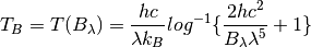
$T_B = T(B_{\lambda}) = \frac{hc}{\lambda k_B} log^{-1}\{\frac{2hc^2}{B_{\lambda} {\lambda}^5} + 1\}$

In python it may look like this:

>>> from pyspectral.blackbody import blackbody_wn_rad2temp
>>> wavenumber = 90909.1
>>> temp = blackbody_wn_rad2temp(wavenumber, [0.001158354, 0.001175477])
>>> print([round(t, 8) for t in temp])
[299.99998562, 301.00000518]

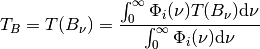
Provided the input is a central wavenumber or wavelength as defined above, this gives the brightness temperature calculation under the assumption of a linear planck function as a function of wavelength or wavenumber over the spectral band width and provided a constant relative spectral response. To get a more precise derivation of the brightness temperature given a measured radiance one needs to convolve the inverse Planck function with the relative spectral response function for the band in question:

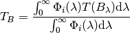
$T_B = \frac{\int_0^\infty \Phi_{i}(\lambda) T(B_{\lambda}) \mathrm{d}\lambda} {\int_0^\infty \Phi_{i}(\lambda) \mathrm{d}\lambda}$

or

$T_B = T(B_{\nu}) = \frac{\int_0^\infty \Phi_{i}(\nu) T(B_{\nu}) \mathrm{d}\nu} {\int_0^\infty \Phi_{i}(\nu) \mathrm{d}\nu}$