Definitions and some radiation theory¶

In radiation physics there is unfortunately several slightly different ways of presenting the theory. For instance, there is no single custom on the mathematical symbolism, and various different non SI-units are used in different situations. Here we present just a few terms and definitions with relevance to PySpectral, and how to possible go from one common representation to another.

Symbols and definitions used in PySpectral¶

$\lambda$

Wavelength ( $\mu m$ )

$\nu = \frac{1}{\lambda}$

Wavenumber ( $cm^{-1}$ )

$\lambda_{c}$

Central wavelength for a given band/channel ( $\mu m$ )

$\nu_{c}$

Central wavelength for a given band/channel ( $cm^{-1}$ )

$\Phi_{i}(\lambda)$

Relative spectral response for band $i$ as a function of wavelength

$E_{\lambda}$

Spectral irradiance at wavelength $\lambda$ ( $W/m^2 \mu m^{-1}$ )

$E_{\nu}$

Spectral irradiance at wavenumber $\nu$ ( $W/m^2 (cm^{-1})^{-1}$ )

$B_{\lambda}$

Blackbody radiation at wavelength $\lambda$ ( $W/m^2 \mu m^{-1}$ )

$B_{\nu}$

Blackbody radiation at wavenumber $\nu$ ( $W/m^2 (cm^{-1})^{-1}$ )

$L_{\nu}$

Spectral radiance at wavenumber $\nu$ ( $W/m^2 sr^{-1} (cm^{-1})^{-1}$ )

$L_{\lambda}$

Spectral radiance at wavelength $\lambda$ ( $W/m^2 sr^{-1} \mu m^{-1}$ )

$L$

Radiance - (band) integrated spectral radiance ( $W/m^2 sr^{-1}$ )

Constants¶

$k_B$

Boltzmann constant ( $1.3806488 1e-23$ )

$h$

Planck constant ( $6.62606957 1e-34$ )

$c$

Speed of light in vacuum ( $2.99792458 1e8$ )

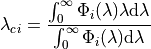
Central wavelength and central wavenumber¶

The central wavelength for a given spectral band ( $i$ ) of a satellite sensor is defined as:

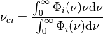
${\lambda_c}_i = \frac{\int_0^\infty \Phi_{i}(\lambda) \lambda \mathrm{d}\lambda} {\int_0^\infty \Phi_{i}(\lambda) \mathrm{d}\lambda}$

Likewise the central wavenumber is:

${\nu_c}_i = \frac{\int_0^\infty \Phi_{i}(\nu) \nu \mathrm{d}\nu} {\int_0^\infty \Phi_{i}(\nu) \mathrm{d}\nu}$

And since $\nu = 1/\lambda$ , we can express the central wavenumber using the spectral response function expressed in wavelength space, as:

${\nu_c}_i = \frac{\int_0^\infty \Phi_{i}(\lambda) \frac{1}{\lambda^{3}} \mathrm{d}\lambda} {\int_0^\infty \Phi_{i}(\lambda) \frac{1}{\lambda^{2}} \mathrm{d}\lambda}$

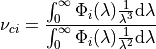
And from this we see that in general $\nu_c \neq 1/\lambda_c$ .

Taking SEVIRI as an example, and looking at the visible channel on Meteosat-8, we see that this is indeed true:

>>> from pyspectral.rsr_reader import RelativeSpectralResponse
>>> from pyspectral.utils import convert2wavenumber, get_central_wave
>>> seviri = RelativeSpectralResponse('Meteosat-8', 'seviri')
>>> cwl = get_central_wave(seviri.rsr['VIS0.6']['det-1']['wavelength'], seviri.rsr['VIS0.6']['det-1']['response'])
>>> print(round(cwl, 6))
0.640216
>>> rsr, info = convert2wavenumber(seviri.rsr)
>>> print("si_scale={scale}, unit={unit}".format(scale=info['si_scale'], unit=info['unit']))
si_scale=100.0, unit=cm-1
>>> wvc = get_central_wave(rsr['VIS0.6']['det-1']['wavenumber'], rsr['VIS0.6']['det-1']['response'])
>>> round(wvc, 3)
15682.622
>>> print(round(1./wvc*1e4, 6))
0.637648

In the PySpectral unified HDF5 formatted spectral response data we also store the central wavelength, so you actually don’t have to calculate them yourself:

>>> from pyspectral.rsr_reader import RelativeSpectralResponse
>>> print("Central wavelength = {cwl}".format(cwl=round(seviri.rsr['VIS0.6']['det-1']['central_wavelength'], 6)))
Central wavelength = 0.640216

Wavelength range¶

Satellite radiometers do not measure outgoing radiance at only the central wavelength, but over a range of wavelengths defined by the spectral response function of the instrument. A given instrument channel is therefore often defined by a wavelength range in the form $\lambda_{min}, \lambda_{c}, \lambda_{max}$ . Where $\lambda_{min}$ and $\lambda_{max}$ are defined by the first and last points in the spectral response function where the response is greater than a given threshold. Pyspectral has a utility function to enable users to compute these wavelength ranges:

>>> from pyspectral.rsr_reader import RelativeSpectralResponse
>>> from pyspectral.utils import get_wave_range
>>> seviri = RelativeSpectralResponse('Meteosat-8', 'seviri')
>>> wvl_range = get_wave_range(seviri.rsr['HRV']['det-1'], 0.15)
>>> print(round(num, 3) for num in wvl_range)
[0.456, 0.715, 0.996]

Spectral Irradiance¶

We denote the spectral irradiance $E$ which is a function of wavelength or wavenumber, depending on what representation is used. In PySpectral the aim is to support both representations. The units are of course dependent of which representation is used.

In wavelength space we write $E(\lambda)$ and it is given in units of $W/m^2 \mu m^{-1}$ .

In wavenumber space we write $E(\nu)$ and it is given in units of $W/m^2 (cm^{-1})^{-1}$ .

To convert a spectral irradiance $E_{\lambda_0}$ at wavelength $\lambda_0$ to a spectral irradiance $E_{\nu_0}$ at wavenumber $\nu_0 = 1/\lambda_0$ the following relation applies:

$E_\nu = E_\lambda \lambda^2$

And if the units are not SI but rather given by the units shown above we have to account for a factor of 10 as:

$E_\nu = {E_\lambda \lambda^2 * 0.1}$

TOA Solar irradiance and solar constant¶

First, the TOA solar irradiance in wavelength space:

>>> from pyspectral.solar import SolarIrradianceSpectrum
>>> solar_irr = SolarIrradianceSpectrum(dlambda=0.0005)
>>> print("Solar irradiance = {}".format(round(solar_irr.solar_constant(), 3)))
Solar irradiance = 1366.091
>>> solar_irr.plot('/tmp/solar_irradiance.png')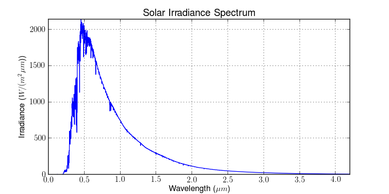

The solar constant is in units of $W/m^2$ . Instead when expressing the irradiance in wavenumber space using wavenumbers in units of $cm^{-1}$ the solar flux is in units of $mW/m^2$ :

>>> solar_irr = SolarIrradianceSpectrum(TOTAL_IRRADIANCE_SPECTRUM_2000ASTM, dlambda=0.0005, wavespace='wavenumber')
>>> print(round(solar_irr.solar_constant(), 5))
1366077.16482
>>> solar_irr.plot('/tmp/solar_irradiance_wnum.png')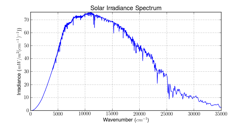

In-band solar flux¶

The solar flux (SI unit $\frac{W}{m^2}$ ) over a spectral sensor band can be derived by convolving the top of atmosphere solar spectral irradiance and the sensor relative spectral response. For band $i$ :

$F_i = \int_0^\infty \Phi_{i}(\lambda) E(\lambda) \mathrm{d}\lambda$

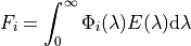
where $E(\lambda)$ is the TOA spectral solar irradiance at a sun-earth distance of one astronomical unit (AU).

In python code it may look like this:

>>> from pyspectral.rsr_reader import RelativeSpectralResponse
>>> from pyspectral.utils import convert2wavenumber, get_central_wave
>>> seviri = RelativeSpectralResponse('Meteosat-8', 'seviri')
>>> rsr, info = convert2wavenumber(seviri.rsr)
>>> from pyspectral.solar import SolarIrradianceSpectrum
>>> solar_irr = SolarIrradianceSpectrum(dlambda=0.0005, wavespace='wavenumber')
>>> print("Solar Irradiance (SEVIRI band VIS008) = {sflux:12.6f}".format(sflux=solar_irr.inband_solarflux(rsr['VIS0.8'])))
Solar Irradiance (SEVIRI band VIS008) = 63767.908405

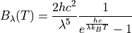
Planck radiation¶

Planck’s law describes the electromagnetic radiation emitted by a black body in thermal equilibrium at a definite temperature.

Thus for wavelength $\lambda$ the Planck radiation or Blackbody radiation $B({\lambda})$ can be written as:

$B_{\lambda}(T) = \frac{2hc^{2}}{{\lambda}^{5}} \frac{1} {e^{\frac{hc}{\lambda k_B T}} - 1}$

and expressed as a function of wavenumber $\nu$ :

$B_{\nu}(T) = 2hc^2{\nu}^3 \frac{1}{e^{\frac{h c \nu}{k_B T}} - 1}$

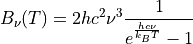
In python it may look like this:

>>> from pyspectral.blackbody import blackbody_wn
>>> wavenumber = 90909.1
>>> rad = blackbody_wn((wavenumber, ), [300., 301])
>>> print("{0:7.6f} {1:7.6f}".format(rad[0], rad[1]))
0.001158 0.001175

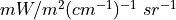Which are the spectral radiances in SI units at wavenumber around $909 cm^{-1}$ at temperatures 300 and 301 Kelvin. In units of $mW/m^2 (cm^{-1})^{-1}\ sr^{-1}$ this becomes:

>>> print("{0:7.4f} {1:7.4f}".format((rad*1e+5)[0], (rad*1e+5)[1]))
115.8354 117.5477

And using wavelength representation:

>>> from pyspectral.blackbody import blackbody
>>> wvl = 1./wavenumber
>>> rad = blackbody(wvl, [300., 301])
>>> print("{0:10.3f} {1:10.3f}".format(rad[0], rad[1]))
9573177.494 9714687.157

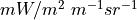Which are the spectral radiances in SI units around $11 \mu m$ at temperatures 300 and 301 Kelvin. In units of $mW/m^2\ m^{-1} sr^{-1}$ this becomes:

>>> print("{0:7.5f} {1:7.5f}".format((rad*1e-6)[0], (rad*1e-6)[1]))
9.57318 9.71469

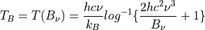
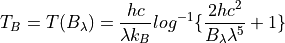
The inverse Planck function¶

Inverting the Planck function allows to derive the brightness temperature given the spectral radiance. Expressed in wavenumber space this becomes:

$T_B = T(B_{\nu}) = \frac{hc\nu}{k_B} log^{-1}\{\frac{2hc^2{\nu}^3}{B_{\nu}} + 1\}$

With the spectral radiance given as a function of wavelength the equation looks like this:

$T_B = T(B_{\lambda}) = \frac{hc}{\lambda k_B} log^{-1}\{\frac{2hc^2}{B_{\lambda} {\lambda}^5} + 1\}$

In python it may look like this:

>>> from pyspectral.blackbody import blackbody_wn_rad2temp
>>> wavenumber = 90909.1
>>> temp = blackbody_wn_rad2temp(wavenumber, [0.001158354, 0.001175477])
>>> print([round(t, 8) for t in temp])
[299.99998562, 301.00000518]

This approach only works for monochromatic or very narrow bands for which the spectral response function is assumed to be constant. In reality, typical imager channels are not that narrow and the spectral response function is not constant over the band. Here it is not possible to de-convolve the planck function and the spectral response function without knowing both, the spectral radiance and spectral response function in high spectral resolution. While this information is usually available for the spectral response function, there is only one integrated radiance per channel. That makes the derivation of brightness temperature from radiance more complicated and more time consuming - in preparation or in execution. Depending on individual requirements, there is a bunch of feasible solutions:

Iterative Method¶

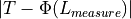
A stepwise approach, which starts with a guess (most common temperature), calculate the radiance that would correspond to that temperature and compare it with the measured radiance. If the difference lies above a certain threshold, adjust the temperature accordingly and start over again:

set uncertainty parameter $\Delta L$

set $T_j = T_{first guess}$

calculate $B(T_j)$

if $(B(T_j) - L_{measure}) > \Delta L$ then adjust $T_j$ and go back to $iii$

$T_j$ matches the measurement within the defined uncertainty

Advantages

no pre-computations
accuracy easily adaptable to purpose
memory friendly
independent of band
independent of spectral response function

Disadvantages

slow, especially when applying to wide bands and high accuracy requirements
redundant calculations when applying to images with many pixels

Function Fit¶

Another feasible approach is to fit a function $\Phi$ in a way that $|T - \Phi(L_{measure})|$ minimizes. This requires pre-calculations of data pairs $T$ and $L(T)$ . Finally an adequate function $\Phi$ (dependent on the shape of $T(L(T))$ ) is assigned and used to calculate the brightness temperature for one channel.

Advantages

fast approach (especially in execution)
minor memory request (one function per channel)

Disadvantages

accuracy determined in the beginning of the process
complexity of $\Phi$ depends on $T(L(T))$

Look-Up Table¶

If the number of possible pairs $T$ and $L(T)$ is limited (e.g. due to limited bit size) or if the setting for a function fit is too complex or does not fit into a processing environment, it is possible to just expand the number of pre-calculated pairs to a look-up table. In an optimal case, the table cover every possible value or is dense enough to allow for linear interpolation.

Advantages

fast approach (but depends on table size)
(almost) independent of function

Disadvantages

accuracy dependent on value density (size of look-up table)
can become a memory issue

Definitions and some radiation theory¶

Symbols and definitions used in PySpectral¶

Constants¶

Central wavelength and central wavenumber¶

Wavelength range¶

Spectral Irradiance¶

TOA Solar irradiance and solar constant¶

In-band solar flux¶

Planck radiation¶

The inverse Planck function¶

Iterative Method¶

Function Fit¶

Look-Up Table¶

Table of Contents

Previous topic

Next topic

This Page

$\lambda$	Wavelength ( $\mu m$ )
$\nu = \frac{1}{\lambda}$	Wavenumber ( $cm^{-1}$ )
$\lambda_{c}$	Central wavelength for a given band/channel ( $\mu m$ )
$\nu_{c}$	Central wavelength for a given band/channel ( $cm^{-1}$ )
$\Phi_{i}(\lambda)$	Relative spectral response for band $i$ as a function of wavelength
$E_{\lambda}$	Spectral irradiance at wavelength $\lambda$ ( $W/m^2 \mu m^{-1}$ )
$E_{\nu}$	Spectral irradiance at wavenumber $\nu$ ( $W/m^2 (cm^{-1})^{-1}$ )
$B_{\lambda}$	Blackbody radiation at wavelength $\lambda$ ( $W/m^2 \mu m^{-1}$ )
$B_{\nu}$	Blackbody radiation at wavenumber $\nu$ ( $W/m^2 (cm^{-1})^{-1}$ )
$L_{\nu}$	Spectral radiance at wavenumber $\nu$ ( $W/m^2 sr^{-1} (cm^{-1})^{-1}$ )
$L_{\lambda}$	Spectral radiance at wavelength $\lambda$ ( $W/m^2 sr^{-1} \mu m^{-1}$ )
$L$	Radiance - (band) integrated spectral radiance ( $W/m^2 sr^{-1}$ )

$k_B$	Boltzmann constant ( $1.3806488 1e-23$ )
$h$	Planck constant ( $6.62606957 1e-34$ )
$c$	Speed of light in vacuum ( $2.99792458 1e8$ )