Derivation of the 3.7 micron reflectance
It is well known that the top of atmosphere signal (observed radiance or
brightness temperature) of a sensor band in the near infrared part of the
spectrum between around  is composed of a thermal (or
emissive) part and a part stemming from reflection of incoming sunlight.
is composed of a thermal (or
emissive) part and a part stemming from reflection of incoming sunlight.
With some assumptions it is possible to separate the two and derive a solar reflectance in the band from the observed brightness temperature. Below we will demonstrate the theory on how this separation is done. But, first we need to demonstrate how the spectral radiance can be calculated from an observed brightness temperature, knowing the relative spectral response of the the sensor band.
Brightness temperature to spectral radiance
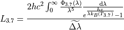
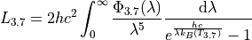
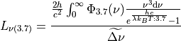
If the satellite observation is given in terms of the brightness temperature, then the corresponding spectral radiance can be derived by convolving the relative spectral response with the Planck function and divding by the equivalent band width:
(1)
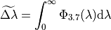
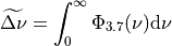
where the equivalent band width  is defined as:
 is the measured radiance at
  ,
,
 is the
  channel
spectral response function, and
channel
spectral response function, and  is the Planck radiation.
This gives the spectral radiance given the brightness temperature and may be
expressed in  , or using SI units
  .
.
>>> from pyspectral.radiance_tb_conversion import RadTbConverter
>>> import numpy as np
>>> sunz = np.array([68.98597217,  68.9865146 ,  68.98705756,  68.98760105, 68.98814508])
>>> tb37 = np.array([298.07385254, 297.15478516, 294.43276978, 281.67633057, 273.7923584])
>>> viirs = RadTbConverter('Suomi-NPP', 'viirs', 'M12')
>>> rad37 = viirs.tb2radiance(tb37)
>>> print([np.round(rad, 7) for rad in rad37['radiance']])
[369717.4972296, 355110.6414922, 314684.3507084, 173143.4836477, 116408.0022674]
>>> rad37['unit']
'W/m^2 sr^-1 m^-1'
In order to get the total radiance over the band one has to multiply with the equivalent band width.
>>> from pyspectral.radiance_tb_conversion import RadTbConverter
>>> import numpy as np
>>> tb37 = np.array([298.07385254, 297.15478516, 294.43276978, 281.67633057, 273.7923584])
>>> viirs = RadTbConverter('Suomi-NPP', 'viirs', 'M12')
>>> rad37 = viirs.tb2radiance(tb37, normalized=False)
>>> print([np.round(rad, 8) for rad in rad37['radiance']])
[0.07037968, 0.06759911, 0.05990353, 0.03295971, 0.02215951]
>>> rad37['unit']
'W/m^2 sr^-1'
By passing normalized=False to the method the division by the equivalent
band width is omitted. The equivalent width is provided as an attribute in SI
units ( ):
):
>>> from pyspectral.radiance_tb_conversion import RadTbConverter
>>> viirs = RadTbConverter('Suomi-NPP', 'viirs', 'M12')
>>> viirs.rsr_integral
1.903607e-07
Inserting the Planck radiation:
(2)
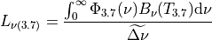
The total band integrated spectral radiance or the in band radiance is then:
(3)
This is expressed in wavelength space. But the spectral radiance can also be
given in terms of the wavenumber  , provided the relative spectral
response is given as a function of :
, provided the relative spectral
response is given as a function of :
where the equivalent band width  is defined as:
and inserting the Planck radiation:
Determination of the in-band solar flux
The solar flux (SI unit  ) over a spectral sensor band can
be derived by convolving the top of atmosphere spectral irradiance and the
sensor relative spectral response curve, so for the band this
would be:
) over a spectral sensor band can
be derived by convolving the top of atmosphere spectral irradiance and the
sensor relative spectral response curve, so for the band this
would be:
(4)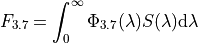
where  is the spectral solar irradiance.
>>> from pyspectral.rsr_reader import RelativeSpectralResponse
>>> from pyspectral.solar import SolarIrradianceSpectrum
>>> viirs = RelativeSpectralResponse('Suomi-NPP', 'viirs')
>>> solar_irr = SolarIrradianceSpectrum(dlambda=0.005)
>>> sflux = solar_irr.inband_solarflux(viirs.rsr['M12'])
>>> print(np.round(sflux, 7))
2.2428119
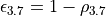
Derive the reflective part of the observed 3.7 micron radiance
The monochromatic reflectivity (or reflectance)  is the
ratio of the reflected (backscattered) radiance to the incident radiance. In
the case of solar reflection one can write:
is the
ratio of the reflected (backscattered) radiance to the incident radiance. In
the case of solar reflection one can write:

where  is the measured radiance,
  is
the incoming solar radiance, and
is
the incoming solar radiance, and  is the cosine of the solar
zenith angle
is the cosine of the solar
zenith angle  .
.
Assuming the solar radiance is independent of direction, the equation for the
reflectance can be written in terms of the solar flux  :
:

For the channel the outgoing radiance is due to solar
reflection and thermal emission. Thus in order to determine a
channel reflectance, it is necessary to subtract the thermal part from the
satellite signal. To do this, the temperature of the observed object is
needed. The usual candidate at hand is the  brightness temperature
(e.g. VIIRS I5 or M12), since most objects behave approximately as blackbodies
in this spectral interval.
brightness temperature
(e.g. VIIRS I5 or M12), since most objects behave approximately as blackbodies
in this spectral interval.
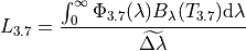
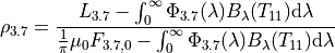
The channel reflectance may then be written as (we now operate
with the in band radiance given by (3))
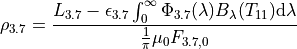
where is the measured radiance at ,
is the channel
spectral response function, is the Planck radiation,
and  is the
  channel brightness temperature.
Observe that is now the radiance provided by (3).
channel brightness temperature.
Observe that is now the radiance provided by (3).
If the observed object is optically thick (transmittance equals zero) then:
and then, with the radiance derived using
(2) and the solar flux given by (4) we get:
(5)
In Python this becomes:
>>> from pyspectral.near_infrared_reflectance import Calculator
>>> import numpy as np
>>> refl_m12 = Calculator('Suomi-NPP', 'viirs', 'M12')
>>> sunz = np.array([68.98597217,  68.9865146 ,  68.98705756,  68.98760105, 68.98814508])
>>> tb37 = np.array([298.07385254, 297.15478516, 294.43276978, 281.67633057, 273.7923584])
>>> tb11 = np.array([271.38806152, 271.38806152, 271.33453369, 271.98553467, 271.93609619])
>>> m12r = refl_m12.reflectance_from_tbs(sunz, tb37, tb11)
>>> print(np.any(np.isnan(m12r)))
False
>>> print([np.round(refl, 6) for refl in m12r])
[0.214329, 0.202852, 0.17064, 0.054089, 0.008381]
We can try decompose equation (5) above using the example of VIIRS M12 band:
>>> from pyspectral.radiance_tb_conversion import RadTbConverter
>>> import numpy as np
>>> sunz = np.array([68.98597217,  68.9865146 ,  68.98705756,  68.98760105, 68.98814508])
>>> tb37 = np.array([298.07385254, 297.15478516, 294.43276978, 281.67633057, 273.7923584])
>>> tb11 = np.array([271.38806152, 271.38806152, 271.33453369, 271.98553467, 271.93609619])
>>> viirs = RadTbConverter('Suomi-NPP', 'viirs', 'M12')
>>> rad37 = viirs.tb2radiance(tb37, normalized=False)
>>> rad11 = viirs.tb2radiance(tb11, normalized=False)
>>> sflux = 2.242817881698326
>>> nomin = rad37['radiance'] - rad11['radiance']
>>> print(np.isnan(nomin))
[False False False False False]
>>> print([np.round(val, 8) for val in nomin])
[0.05083677, 0.0480562, 0.04041571, 0.01279277, 0.00204485]
>>> denom = np.cos(np.deg2rad(sunz))/np.pi * sflux - rad11['radiance']
>>> print(np.isnan(denom))
[False False False False False]
>>> print([np.round(val, 8) for val in denom])
[0.23646312, 0.23645681, 0.23650559, 0.23582014, 0.23586609]
>>> res = nomin/denom
>>> print(np.isnan(res))
[False False False False False]
>>> print([np.round(val, 8) for val in res])
[0.21498817, 0.20323458, 0.17088693, 0.05424801, 0.00866952]
Derive the emissive part of the 3.7 micron band
Now that we have the reflective part of the  signal, it is easy to derive
the emissive part, under the same assumptions of completely opaque (zero
transmissivity) objects.
signal, it is easy to derive
the emissive part, under the same assumptions of completely opaque (zero
transmissivity) objects.
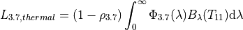
Using the example of the VIIRS M12 band from above this gives the following spectral radiance:
>>> from pyspectral.near_infrared_reflectance import Calculator
>>> import numpy as np
>>> refl_m12 = Calculator('Suomi-NPP', 'viirs', 'M12')
>>> sunz = np.array([68.98597217,  68.9865146 ,  68.98705756,  68.98760105, 68.98814508])
>>> tb37 = np.array([298.07385254, 297.15478516, 294.43276978, 281.67633057, 273.7923584])
>>> tb11 = np.array([271.38806152, 271.38806152, 271.33453369, 271.98553467, 271.93609619])
>>> m12r = refl_m12.reflectance_from_tbs(sunz, tb37, tb11)
>>> tb = refl_m12.emissive_part_3x()
>>> ['{tb:6.3f}'.format(tb=np.round(t, 4)) for t in tb]
['266.996', '267.262', '267.991', '271.033', '271.927']
>>> rad = refl_m12.emissive_part_3x(tb=False)
>>> ['{rad:6.1f}'.format(rad=np.round(r, 1)) for r in rad.compute()]
['80285.2', '81458.0', '84749.7', '99761.4', '104582.0']